# functioon for building model and guide with covariates and K states
def make_hmm_model_and_guide_cov(K):
@config_enumerate
def model(obs, x_pi, x_A, x_em):
# forza obs a torch.Tensor
obs = torch.as_tensor(obs)
N, T = obs.shape
C_pi = x_pi.shape[1]
C_A = x_A.shape[2]
C_em = x_em.shape[2]
# Priors
alpha_pi = 0.5 * torch.ones(K) # <1 → più “spiky”
alpha_A = torch.full((K, K), 0.5)
alpha_A.fill_diagonal_(6.0) # forte massa in diagonale
pi_base = pyro.sample("pi_base", dist.Dirichlet(alpha_pi)) # [K]
A_base = pyro.sample("A_base", dist.Dirichlet(alpha_A).to_event(1)) # [K,K]
log_pi_base = pi_base.log()
log_A_base = A_base.log()
# Parametri globali
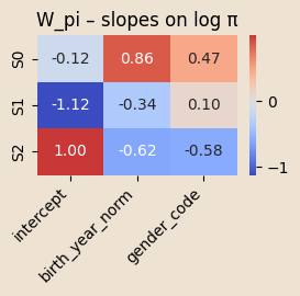
W_pi = pyro.param("W_pi", 0.01 * torch.randn(K, C_pi))
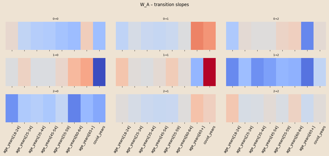
W_A = pyro.param("W_A", 0.01 * torch.randn(K, K, C_A))
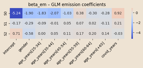
beta_em = pyro.param("beta_em", 0.01 * torch.randn(K, C_em))
with pyro.plate("seqs", N):
# stato iniziale
logits0 = log_pi_base + (x_pi @ W_pi.T)
z_prev = pyro.sample("z_0", dist.Categorical(logits=logits0),
infer={"enumerate": "parallel"})
log_mu_0 = (x_em[:, 0, :] * beta_em[z_prev, :]).sum(-1)
pyro.sample("y_0", dist.Poisson(log_mu_0.exp()), obs=obs[:, 0])
# transizioni
for t in range(1, T):
x_t = x_A[:, t, :]
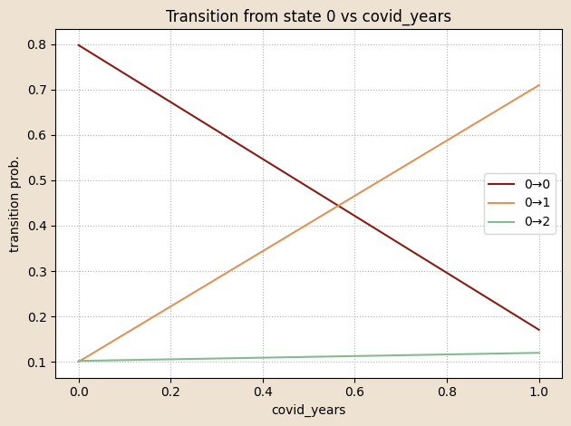
logitsT = (log_A_base[z_prev] + (W_A[z_prev] * x_t[:, None, :]).sum(-1))
z_t = pyro.sample(f"z_{t}", dist.Categorical(logits=logitsT),
infer={"enumerate": "parallel"})
log_mu_t = (x_em[:, t, :] * beta_em[z_t, :]).sum(-1)
pyro.sample(f"y_{t}", dist.Poisson(log_mu_t.exp()), obs=obs[:, t])
z_prev = z_t
def guide(obs, x_pi, x_A, x_em):
# forza obs a torch.Tensor
obs = torch.as_tensor(obs)
# Parametri MAP per pi e A
pi_q = pyro.param("pi_base_map",
torch.ones(K) / K,
constraint=dist.constraints.simplex)
A_init = torch.eye(K) * (K - 1.) + 1.
A_init = A_init / A_init.sum(-1, keepdim=True)
A_q = pyro.param("A_base_map",
A_init,
constraint=dist.constraints.simplex)
pyro.sample("pi_base", dist.Delta(pi_q).to_event(1))
pyro.sample("A_base", dist.Delta(A_q).to_event(2))
#num_params = K * x_pi.shape[1] + K * K * x_A.shape[2] + K * (x_em.shape[2] + 1) + K + K*K
return model, guide
# Reads the variational parameters from the ParamStore and returns point estimates.
@torch.no_grad()
def extract_posterior_point_estimates_cov():
store = pyro.get_param_store()
def softmax_row(v):
e = np.exp(v - np.max(v, axis=-1, keepdims=True))
return e / e.sum(axis=-1, keepdims=True)
# 1) Extract learned parameters
pi_base = pyro.param("pi_base_map").detach().cpu().numpy() # (K,) simplex
A_base = pyro.param("A_base_map").detach().cpu().numpy() # (K, K) rows on simplex
W_pi = pyro.param("W_pi").detach().cpu().numpy() # (K, C_pi)
W_A = pyro.param("W_A").detach().cpu().numpy() # (K, K, C_A)
beta_em = pyro.param("beta_em").detach().cpu().numpy() # (K, 1 + C_em) if intercept first
# 2) Covariate means
x_mean_pi = cov_init_torch.mean(dim=0).detach().cpu().numpy() # (C_pi,)
x_mean_A = cov_tran_torch.mean(dim=(0, 1)).detach().cpu().numpy() # (C_A,)
x_mean_em = cov_emiss_torch.mean(dim=(0,1)).detach().cpu().numpy() # (C_em,)
# 3) Mean initial probs, transitions and rates under average covariates
logits_pi = np.log(pi_base + 1e-30) + W_pi @ x_mean_pi
pi_mean = softmax_row(logits_pi[None, :]).ravel()
K = pi_mean.shape[0]
A_mean = np.zeros((K, K))
for k in range(K):
logits_row = np.log(A_base[k] + 1e-30) + (W_A[k] @ x_mean_A)
A_mean[k] = softmax_row(logits_row[None, :]).ravel()
rates_mean = np.zeros(K)
for k in range(K):
log_mu = np.dot(x_mean_em, beta_em[k, :])
rates_mean[k] = np.exp(log_mu)
return pi_mean, A_mean, rates_mean
# Uses the learned parameters from the ParamStore to make predictions on test data, compute MSE and Accuracy, and display a plot."
def evaluate_hmm_glm_prediction(obs_test, xpi_test, xA_test, xem_test):
store = pyro.get_param_store()
def softmax_row(v):
e = np.exp(v - np.max(v, axis=-1, keepdims=True))
return e / e.sum(axis=-1, keepdims=True)
# 1) Extract learned parameters
pi_base = pyro.param("pi_base_map").detach().cpu().numpy() # (K,)
A_base = pyro.param("A_base_map").detach().cpu().numpy() # (K, K)
W_pi = pyro.param("W_pi").detach().cpu().numpy() # (K, C_pi)
W_A = pyro.param("W_A").detach().cpu().numpy() # (K, K, C_A)
beta_em = pyro.param("beta_em").detach().cpu().numpy() # (K, 1 + C_em)
# 2) Convert test data to NumPy
obs_test_np = obs_test.detach().cpu().numpy()
xpi_test_np = xpi_test.detach().cpu().numpy()
xA_test_np = xA_test.detach().cpu().numpy()
xem_test_np = xem_test.detach().cpu().numpy()
# 3) One-step ahead prediction
y_pred_hmm, state_prob = hmm_forward_predict(
obs_so_far=obs_test_np[:, :-1],
xpi=xpi_test_np,
xA=xA_test_np,
A_base=A_base,
W_pi=W_pi,
W_A=W_A,
pi_base=pi_base,
beta_em=beta_em,
cov_emission=xem_test_np,
steps_ahead=1
)
# 4) True values
y_test = obs_test_np[:, -1]
# 5) Compute metrics
mse = np.mean((y_pred_hmm - y_test)**2)
acc = 100*np.mean(np.round(y_pred_hmm) == y_test)
print(f"HMM(full): pred mean={y_pred_hmm.mean():.2f} obs mean={y_test.mean():.2f}")
print(f"MSE: {mse:.4f}")
return y_pred_hmm, y_test, mse, acc
# def log_softmax_logits(logits, dim=-1):
# return logits - torch.logsumexp(logits, dim=dim, keepdim=True)
# Computes the forward algorithm log-likelihood for a covariate-dependent HMM with Poisson emissions using the parameters stored in the Pyro ParamStore.
@torch.no_grad()
def forward_loglik_cov(obs, x_pi, x_A, x_em):
device = obs.device
ps = pyro.get_param_store()
pi_base = ps["pi_base_map"].to(device)
A_base = ps["A_base_map"].to(device)
W_pi = ps["W_pi"].to(device)
W_A = ps["W_A"].to(device)
beta_em = ps["beta_em"].to(device)
N, T = obs.shape
K = pi_base.shape[0]
B = beta_em[:, :]
log_mu = torch.einsum("ntc,kc->ntk", x_em.to(device), B)
emis_log = dist.Poisson(rate=log_mu.exp()).log_prob(obs.unsqueeze(-1)) # (N,T,K)
log_pi = log_softmax_logits(pi_base.log() + x_pi @ W_pi.T, dim=1) # (N,K)
log_alpha = log_pi + emis_log[:, 0]
log_A0 = A_base.log()
for t in range(1, T):
x_t = x_A[:, t, :]
logits = log_A0.unsqueeze(0) + (W_A.unsqueeze(0) * x_t[:, None, None, :]).sum(-1)
log_A = log_softmax_logits(logits, dim=2)
log_alpha = torch.logsumexp(log_alpha.unsqueeze(2) + log_A, dim=1) + emis_log[:, t]
return torch.logsumexp(log_alpha, dim=1) # (N,)
# Evaluate HMM-GLM models with different numbers of latent states, evaluates them using log-evidence and prediction accuracy
def train_and_evaluate_cov(obs_torch, x_pi, x_A, x_em, K_list, n_steps=500, lr=1e-5):
log_evidences = []
final_elbos = [] # salvo gli ELBO finali
accuracies = [] # salvo le accuracy
for K in K_list:
print(f"\n=== Training HMM with K={K} states ===")
# crea modello e guida
model, guide = make_hmm_model_and_guide_cov(K)
# resetta ParamStore
pyro.clear_param_store()
svi = SVI(model, guide,
Adam({"lr": lr}),
loss=TraceEnum_ELBO(max_plate_nesting=1))
losses = []
for step in range(n_steps):
loss = svi.step(obs_torch, x_pi, x_A, x_em)
losses.append(loss)
if step % 50 == 0:
print(f"K={K} | step {step:4d} ELBO = {loss:,.0f}")
# ELBO finale
final_elbo_val = -losses[-1]
final_elbos.append(final_elbo_val)
# 🔹 calcolo metriche di prediction (inclusa accuracy)
_, _, mse, acc = evaluate_hmm_glm_prediction(obs_torch, x_pi, x_A, x_em)
accuracies.append(acc)
# calcola log-likelihood / evidenza
log_evidence_val = forward_loglik_cov(obs_torch, x_pi, x_A, x_em).sum()
log_evidences.append(log_evidence_val)
print(f"Log-evidence K={K}: {log_evidence_val:.2f}")
print(f"Accuracy K={K}: {acc:.2f}%")
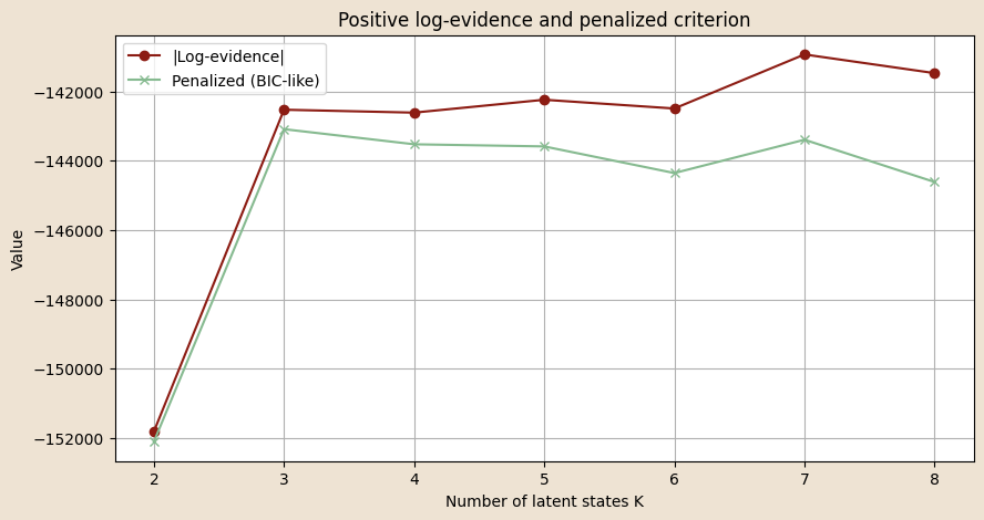
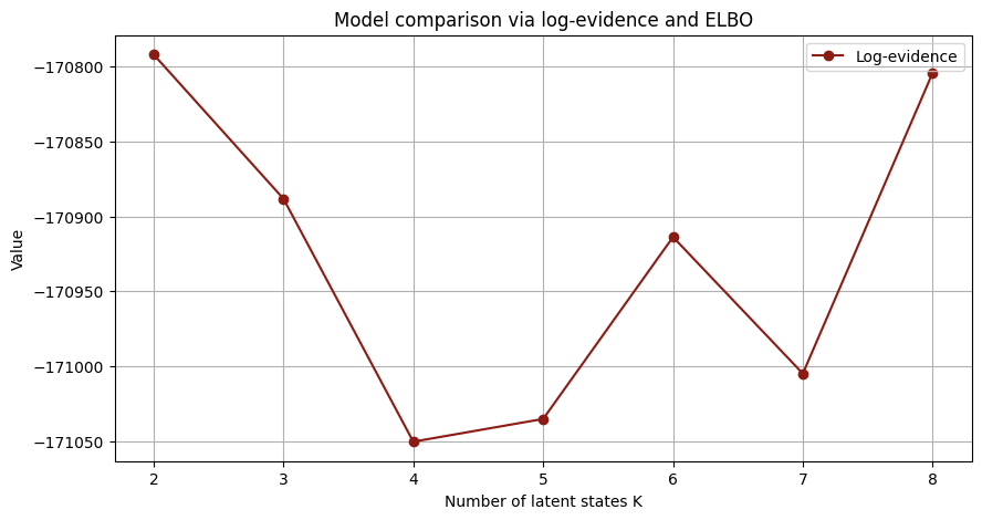
# 🔹 Plot evidenze e ELBO
plt.figure(figsize=(10,5))
plt.plot(K_list, log_evidences, marker='o', label="Log-evidence")
#plt.plot(K_list, final_elbos, marker='x', label="Final ELBO")
plt.xlabel("Number of latent states K")
plt.ylabel("Value")
plt.title("Model comparison via log-evidence and ELBO")
plt.legend()
plt.grid(True)
plt.show()
# 🔹 Plot accuracy come istogramma
plt.figure(figsize=(8,5))
plt.bar([str(K) for K in K_list], accuracies, color="skyblue")
plt.xlabel("Number of latent states K")
plt.ylabel("Accuracy (%)")
plt.title("Prediction Accuracy by Model (HMM-GLM)")
plt.grid(axis="y", linestyle="--", alpha=0.7)
# settaggio asse y
y_min = 30
y_max = max(accuracies) + 2 # così lasci un po’ di margine sopra
plt.ylim(y_min, y_max)
plt.yticks(np.arange(y_min, y_max+1, 2)) # tick ogni 2
plt.show()
return K_list, log_evidences, final_elbos, accuracies